(1) Simulate responses and response times based on the HMDCM model with response times (no covariance between speed and learning ability)
class_0 <- sample(1:2^K, N, replace = L)
Alphas_0 <- matrix(0,N,K)
for(i in 1:N){
  Alphas_0[i,] <- inv_bijectionvector(K,(class_0[i]-1))
}
thetas_true = rnorm(N,0,1)
tausd_true=0.5
taus_true = rnorm(N,0,tausd_true)
G_version = 3
phi_true = 0.8
lambdas_true <- c(-2, 1.6, .4, .055)       # empirical from Wang 2017
Alphas <- sim_alphas(model="HO_sep",
                    lambdas=lambdas_true,
                    thetas=thetas_true,
                    Q_matrix=Q_matrix,
                    Design_array=Design_array)
table(rowSums(Alphas[,,5]) - rowSums(Alphas[,,1])) # used to see how much transition has taken place
#>
#>   0   1   2   3   4
#>  62  56  90 116  26
itempars_true <- matrix(runif(J*2,.1,.2), ncol=2)
RT_itempars_true <- matrix(NA, nrow=J, ncol=2)
RT_itempars_true[,2] <- rnorm(J,3.45,.5)
RT_itempars_true[,1] <- runif(J,1.5,2)

Y_sim <- sim_hmcdm(model="DINA",Alphas,Q_matrix,Design_array,
                   itempars=itempars_true)
L_sim <- sim_RT(Alphas,Q_matrix,Design_array,RT_itempars_true,taus_true,phi_true,G_version)
(2) Run the MCMC to sample parameters from the posterior distribution
output_HMDCM_RT_sep = hmcdm(Y_sim,Q_matrix,"DINA_HO_RT_sep",Design_array,
                            100, 30,
                            Latency_array = L_sim, G_version = G_version,
                            theta_propose = 2,deltas_propose = c(.45,.35,.25,.06))
#> 0
output_HMDCM_RT_sep
#>
#> Model: DINA_HO_RT_sep
#>
#> Sample Size: 350
#> Number of Items:
#> Number of Time Points:
#>
#> Chain Length: 100, burn-in: 50
summary(output_HMDCM_RT_sep)
#>
#> Model: DINA_HO_RT_sep
#>
#> Item Parameters:
#>  ss_EAP  gs_EAP
#>  0.1537 0.15645
#>  0.2234 0.17700
#>  0.1617 0.10349
#>  0.1660 0.13320
#>  0.1672 0.04867
#>    ... 45 more items
#>
#> Transition Parameters:
#>    lambdas_EAP
#> λ0     -2.8233
#> λ1      2.8569
#> λ2      0.1297
#> λ3      0.2263
#>
#> Class Probabilities:
#>      pis_EAP
#> 0000 0.09633
#> 0001 0.11772
#> 0010 0.15828
#> 0011 0.28949
#> 0100 0.20747
#>    ... 11 more classes
#>
#> Deviance Information Criterion (DIC): 158380
#>
#> Posterior Predictive P-value (PPP):
#> M1: 0.5096
#> M2:  0.49
#> total scores:  0.6255
a <- summary(output_HMDCM_RT_sep)
head(a$ss_EAP)
#>           [,1]
#> [1,] 0.1537268
#> [2,] 0.2233809
#> [3,] 0.1616863
#> [4,] 0.1659806
#> [5,] 0.1672054
#> [6,] 0.2223146
(3) Check for parameter estimation accuracy
(cor_thetas <- cor(thetas_true,a$thetas_EAP))
#>           [,1]
#> [1,] 0.8005269
(cor_taus <- cor(taus_true,a$response_times_coefficients$taus_EAP))
#>           [,1]
#> [1,] 0.9865148

(cor_ss <- cor(as.vector(itempars_true[,1]),a$ss_EAP))
#>           [,1]
#> [1,] 0.7161335
(cor_gs <- cor(as.vector(itempars_true[,2]),a$gs_EAP))
#>        [,1]
#> [1,] 0.7148

AAR_vec <- numeric(L)
for(t in 1:L){
  AAR_vec[t] <- mean(Alphas[,,t]==a$Alphas_est[,,t])
}
AAR_vec
#> [1] 0.9092857 0.9192857 0.9342857 0.9521429 0.9485714

PAR_vec <- numeric(L)
for(t in 1:L){
  PAR_vec[t] <- mean(rowSums((Alphas[,,t]-a$Alphas_est[,,t])^2)==0)
}
PAR_vec
#> [1] 0.6771429 0.7200000 0.7771429 0.8342857 0.8285714
(4) Evaluate the fit of the model to the observed response and response times data (here, Y_sim and R_sim)
a$DIC
#> Transition Response_Time Response Joint Total
#> D_bar 1895.903 136977.0 15190.81 3165.161 157228.9
#> D(theta_bar) 1589.576 136533.7 14847.80 3106.744 156077.8
#> DIC 2202.230 137420.3 15533.82 3223.578 158380.0
head(a$PPP_total_scores)
#> [,1] [,2] [,3] [,4] [,5]
#> [1,] 0.22 0.30 0.28 0.94 0.94
#> [2,] 0.76 0.90 0.46 0.46 0.12
#> [3,] 0.66 0.34 0.92 0.52 0.24
#> [4,] 0.42 0.40 0.84 0.74 0.56
#> [5,] 0.26 0.82 0.26 0.46 0.62
#> [6,] 0.78 0.82 0.18 0.74 0.64
head(a$PPP_item_means)
#> [1] 0.48 0.58 0.46 0.58 0.52 0.58
head(a$PPP_item_ORs)
#> [,1] [,2] [,3] [,4] [,5] [,6] [,7] [,8] [,9] [,10] [,11] [,12] [,13] [,14]
#> [1,] NA 0.74 0.96 0.96 0.66 0.44 0.78 0.66 0.78 0.88 0.90 0.70 0.94 0.08
#> [2,] NA NA 0.78 1.00 0.68 0.86 0.82 0.96 0.68 0.80 0.64 0.68 0.14 0.62
#> [3,] NA NA NA 0.08 0.82 0.28 0.66 0.64 0.34 0.96 0.20 0.84 0.44 0.84
#> [4,] NA NA NA NA 0.84 1.00 0.94 0.90 0.94 0.92 0.78 0.52 0.02 0.36
#> [5,] NA NA NA NA NA 0.66 0.66 0.78 0.70 0.92 0.90 0.56 0.88 0.16
#> [6,] NA NA NA NA NA NA 0.60 0.54 0.86 0.26 0.82 0.00 0.78 0.28
#> [,15] [,16] [,17] [,18] [,19] [,20] [,21] [,22] [,23] [,24] [,25] [,26]
#> [1,] 0.54 0.84 0.96 0.80 0.64 0.72 0.94 1.00 0.92 0.40 0.14 0.92
#> [2,] 0.74 0.82 0.68 0.66 0.90 0.92 0.02 0.70 0.68 0.62 0.88 0.74
#> [3,] 0.72 0.96 0.62 0.66 0.94 1.00 0.70 0.60 0.46 0.90 0.96 0.98
#> [4,] 0.92 0.98 1.00 0.80 0.90 0.68 0.76 0.24 0.54 0.80 0.98 1.00
#> [5,] 0.18 0.82 0.58 0.50 0.82 0.44 0.60 0.82 0.94 0.18 1.00 1.00
#> [6,] 0.74 0.50 0.62 0.90 1.00 0.88 0.10 0.70 0.72 0.70 0.92 0.60
#> [,27] [,28] [,29] [,30] [,31] [,32] [,33] [,34] [,35] [,36] [,37] [,38]
#> [1,] 0.94 0.40 1.00 0.52 0.98 0.54 0.36 0.64 0.86 0.76 0.58 0.92
#> [2,] 0.82 0.92 0.24 0.70 0.26 0.48 0.10 0.68 0.38 0.88 0.08 0.36
#> [3,] 0.38 0.50 0.96 0.80 0.54 0.28 0.18 0.02 0.20 1.00 0.74 0.92
#> [4,] 0.04 1.00 0.96 0.84 0.92 0.38 0.24 0.86 0.94 0.54 0.92 0.88
#> [5,] 0.50 0.34 0.86 0.98 0.74 0.96 0.82 0.92 0.48 0.98 0.28 0.78
#> [6,] 0.86 0.76 0.14 0.86 0.38 0.40 0.82 0.98 0.86 0.66 0.48 0.32
#> [,39] [,40] [,41] [,42] [,43] [,44] [,45] [,46] [,47] [,48] [,49] [,50]
#> [1,] 1.00 0.26 0.62 0.08 0.58 0.70 0.16 0.34 0.82 0.68 0.78 0.38
#> [2,] 0.68 0.76 0.16 1.00 0.76 0.34 0.18 0.50 0.38 0.66 0.44 0.74
#> [3,] 0.74 0.62 0.50 0.32 0.70 1.00 0.76 0.22 0.60 0.34 0.62 0.56
#> [4,] 0.18 0.50 0.10 0.48 0.12 0.98 0.12 0.52 0.12 0.92 0.68 0.52
#> [5,] 0.90 0.58 0.76 0.30 0.68 0.98 0.12 0.16 0.82 0.12 0.56 0.70
#> [6,] 0.80 0.70 0.80 0.90 0.24 0.38 0.10 0.22 0.16 0.58 0.64 0.52
library(bayesplot)
#> This is bayesplot version 1.15.0
#> - Online documentation and vignettes at mc-stan.org/bayesplot
#> - bayesplot theme set to bayesplot::theme_default()
#> * Does _not_ affect other ggplot2 plots
#> * See ?bayesplot_theme_set for details on theme setting
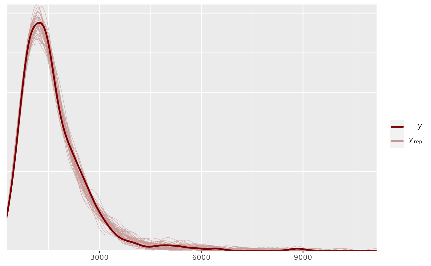
pp_check(output_HMDCM_RT_sep, type="total_latency")